|
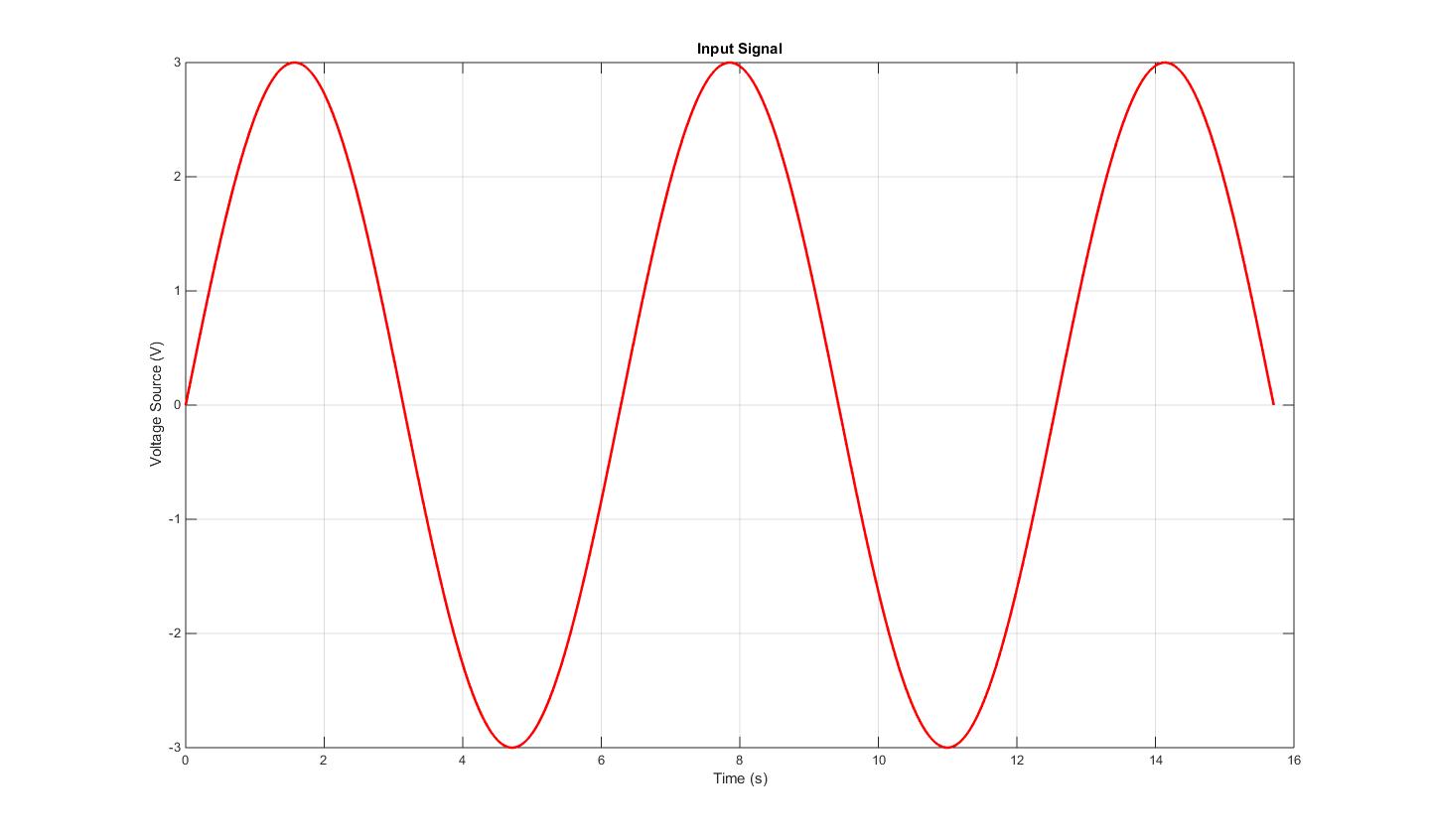
What is a Signal? A signal is a set of data or information. In general, signals are functions of the independent variable time. This is not always the case, however. When an electrical charge is distributed over a body, for instance, the signal is the charge density, a function of space rather than time. The term "signal" includes, among others, audio, video, speech, image, communication, geophysical, sonar, radar, medical and musical signals. Some examples of signals are: a telephone or a television signal, monthly sales of a corporation, or daily closing prices of a stock market (e.g., the Dow Jones averages), a sinusoidal voltage source (the AC voltage outlets), a sound wave being produced when you pluck a guitar string, your heart rate (plotted on an electrocardiogram), temperature in a room throughout the day, and more. In the real world, signals are not always regular and periodic like a sine or cosine wave for example. They can be very complicated, aperiodic and irregular (think of an electrocardiogram). Below is a sine wave that could represent a voltage source to a circuit. Click to change to a non-periodic signal:
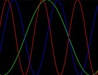
Sinusoidal Signals Periodic signals are those signals that repeat in time with a certain period. Sinusoidal signals are very important because (as we will see below) they can be used to represent any periodic signal. Sinusoidal signals have 3 parameters: amplitude, frequency and phase. The amplitude determines the highest value the signal reaches. The frequency determines how often a signal goes through a cycle (repeats). The phase of a signal determines where the signal starts compared to its "parent function". For example, determine the amplitude, frequency and phase of the following signal which is a function of time: $$x(t) = 3sin(4\pi t+30 \,^{\circ}) $$To visualize signals better and understand how the parameters mentioned above shape the signal, let's try the following example. Manipulate the frequency and amplitude of the sine wave to see what happens to it: Signal Transformations As you see in the above example, changing the signal's frequency or amplitude changes it's behaviour and shape. We can say the signal has been "transformed" from a primitive (sine) signal to
a more complex one. The main transformations of time that we can perform on signals are: For example, let's say: $$x(t) = cos(t - \tau)$$
How will changing Tau affect x(t)? Change Tau below to see the effect: For positive values of Tau, increasing Tau expands the signal in time. For negative Tau, the signal time-reverses and decreasing Tau expands the signal in time.
The above example where you could change the frequency gives you an idea of the effect in this case. However, below is an example of time reversal that happens when Tao becomes negative: Signal Energy Signals, as you saw above, can have positive or negative values for different time intervals. If we considered a signal's area as a positive measure of its size,
because it takes into account both the amplitude and duration of the signal, we will soon run into a problem. The positive and negative areas could cancel each other and result in an inaccurate size.
This difficulty can be corrected by defining the signal size as the area under x2(t), which is always positive. We call this measure the signal energy Ex:
$$E_{x} = \int_{-\infty}^{\infty}|x(t)|^{2}dt$$
Let's take for example a simple signal such as x(t) = sin(t) from 0 to t. To find its Energy, we first need to square the signal to get x2(t) = sin2(t).
Below is a graphical representation of this squared signal sin2(t). Hover over the graph to see the area from 0 to that point which will indicate the energy. Notice how the energy
increases as t increases:
Fourier Series A Fourier series is a way to represent a wave-like function as the sum of simple sine waves. More formally,
it decomposes any periodic function or periodic signal into the sum of a (possibly infinite) set of simple oscillating functions, namely sines and cosines (or, equivalently, complex
exponentials).
Image from: http://www.stewartcalculus.com/
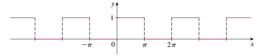
Then we can easily calculate a0, an and bn by using the formulas above: $$a_0 = \frac{1}{2\pi}\int_{-\pi}^{\pi}x(t)dt= \frac{1}{2} \hspace{0.8 in} a_n = \frac{1}{\pi}\int_{-\pi}^{\pi}x(t)cos(nt)dt= \frac{1}{n\pi}[sin(n\pi)-sin(0)]=0$$ $$b_n = \frac{1}{\pi}\int_{-\pi}^{\pi}x(t)sin(nt)dt=\frac{1}{\pi}\int_{-\pi}^{0}0\,dt + \frac{1}{\pi}\int_{0}^{\pi}sin(t)\,dt = \left\{\begin{matrix} 0 \hspace{1 cm} if \,\,n \,\,is\,\,even& \\ \frac{2}{n\pi} \hspace{1 cm} if \,\,n \,\,is\,\,odd& \end{matrix}\right.$$ Approximating a Square Wave using a Fourier Series: Using the same method as in the exercise above, we can derive this formula to approximate a square wave: $$x_{square}(t) = \frac{4}{\pi} \sum_{k=1}^{\infty} (-1)^k \frac{sin(2\pi(2k-1)ft)}{2k-1}$$ To give a better idea of how the Fourier Series works visually, consider the following example (note: this square wave oscillates about the x-axis): Approximating a Triangle Wave using a Fourier Series: Here is the formula for approximating a triangle wave. This formula can be derived using the above exercise. $$x_{triangle}(t) = \frac{8}{\pi^2} \sum_{k=0}^{\infty} (-1)^k \frac{sin(2\pi(2k+1)ft)}{(2k+1)^2}$$Approximating a Sawtooth Wave using a Fourier Series: Here is the formula for approximating a sawtooth wave: $$x_{sawtooth}(t) = \frac{2}{\pi} \sum_{k=1}^{\infty} (-1)^k \frac{sin(2\pi kft)}{k}$$Signal Sampling
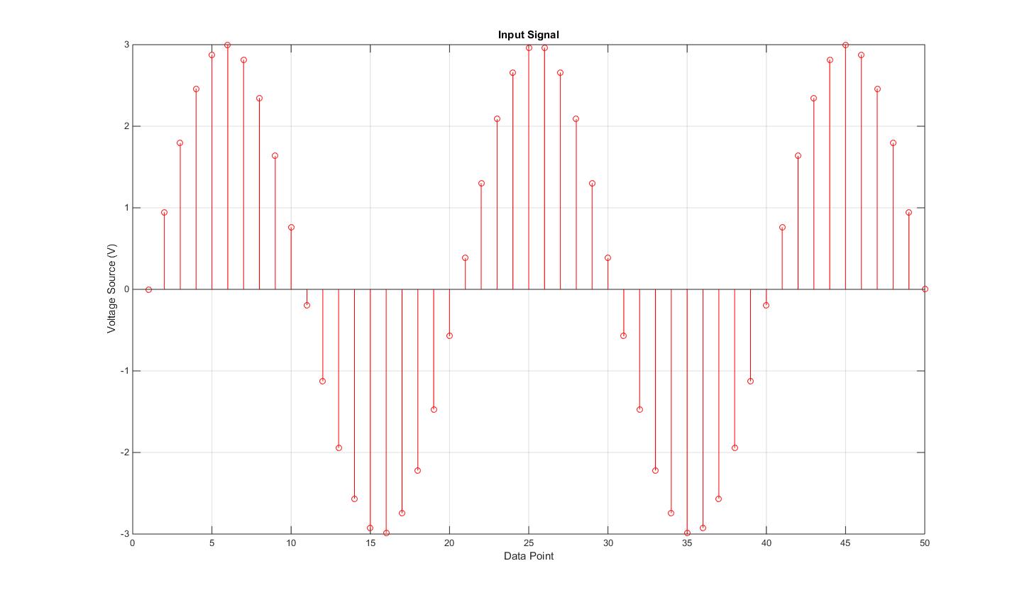
Here is an example of a sine wave sampled every 0.5 seconds. It is clear that as the sampling frequency goes to infinity, we get an exact reconstruction of our original sine wave.
References
|
|||||||||||||
|
|
||||||||||||||